Topics:
- Oscilloscope introduction
- Picoscope introduction
- Picoscope: setting the voltage
- Picoscope: setting the time per division
- Picoscope: setting the trigger
- Picoscope: scale and offset
- Fluke: introduction
- Fluke: setting the zero line
- Fluke: setting the voltage and time per division
- Fluke: setting the trigger
- Fluke: enabling or disabling the smooth function
- Fluke: enabling channel B
- Fluke: measuring with the current clamp
Oscilloscope introduction:
An oscilloscope (abbreviated as “scope”) is a graphical voltmeter that displays voltage as a function of time. The oscilloscope is very accurate and can set the time scale so small that signals can be analyzed precisely. An oscilloscope cannot measure current like a multimeter can up to 400 mA or 10 amperes. To measure current, a current clamp must be used that measures the magnetic field strength around a wire.
Picoscope introduction:
An oscilloscope is indispensable for diagnosing complex faults. There are different variants of the oscilloscope: integrated into the scan tool (e.g. with Snap-on or dealer diagnostic equipment), a handheld oscilloscope (Fluke, also described on this page) and versions that can be connected to a computer / laptop.
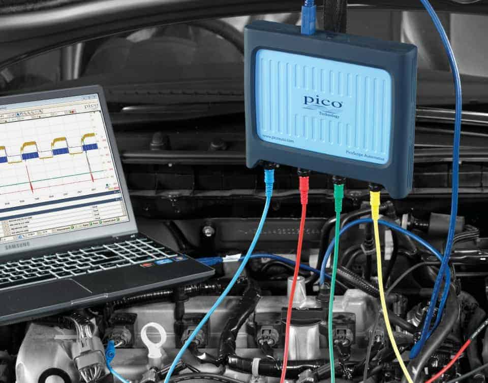
The latter applies to the Picoscope. The hardware of this scope is built into a small housing that can be connected via a USB 2.0 or 3.0 (printer) cable to a computer running the Windows or Macintosh operating system.
On the computer we use the Picoscope software. The hardware of the scope unlocks various functions in the software; a more advanced (and more expensive) scope can therefore do more in software than an entry-level version. The image shows the Automotive (4000-series) scope.
The following sections describe the basic settings for measurements with the Picoscope.
There are different versions of the Picoscope. In automotive use, the following types, among others, may be of interest:
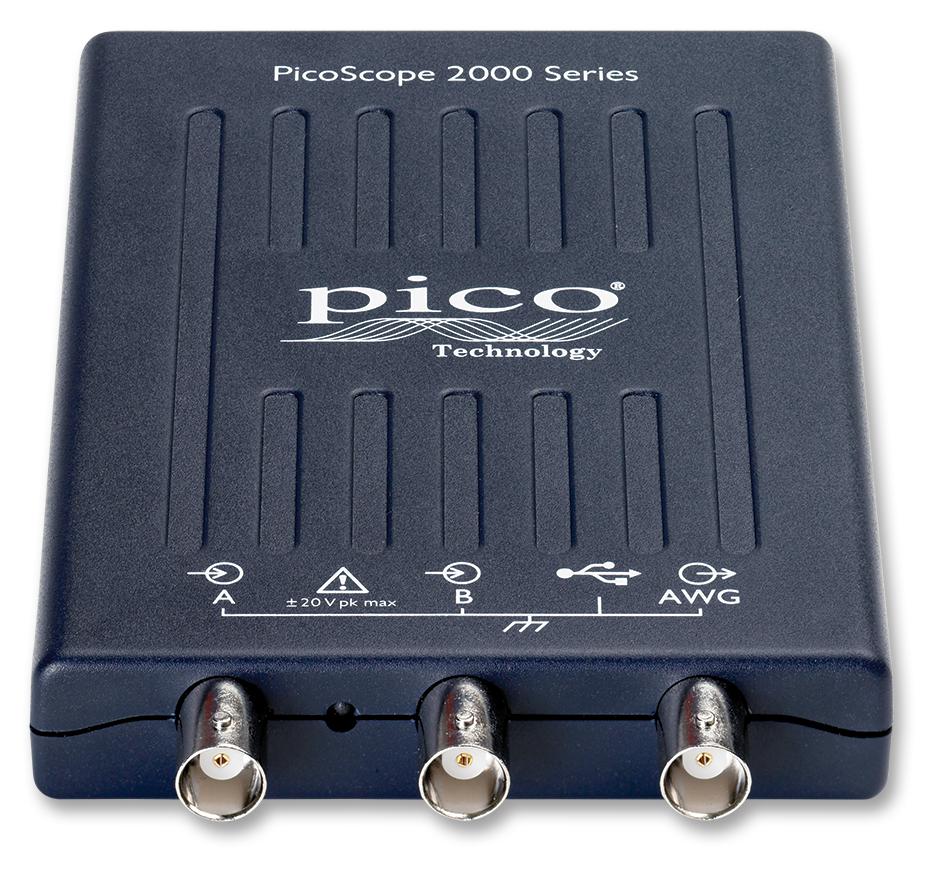
Picoscope 2204a:
The Picoscope 2204A is already available from €130 and is suitable for most automotive applications. The purchase price is attractive, but you need to take the following into account:
- The grounds of channel A and B are internally connected. During a two-channel measurement there is no issue if the ground leads are connected to a ground point on the vehicle. However, if during a two-channel measurement a voltage is present on one of the ground leads, a short circuit will occur in the oscilloscope. The hardware will be damaged;
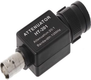
- The measurement range is from -20 to 20 volts. For measuring a PWM signal or CAN bus this is more than sufficient, but if a higher voltage must be measured, e.g. the inductive peak of an injector, an extra accessory must be used: a so‑called “attenuator”. This reduces the measured and displayed voltage by a factor of 20. If 60 volts is measured, this voltage will be shown as 3 volts;
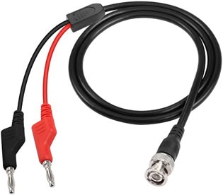
- Personally I do not like the supplied cable set. I prefer to use alternative BNC test leads;
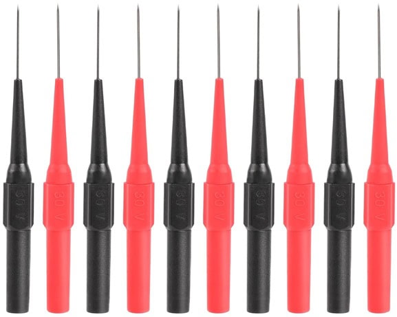
- Probe needles and crocodile clips make it easy to measure in connectors or to connect to positive or ground points.

Tips for purchasing these accessories:
- Picoscope 2204 option 1 or option 2 without standard test leads
- Hantek HT201 attenuator 20:1 (Dutch webshop) or via Aliexpress
- Test leads with BNC connectors option 1 with banana plugs, option 2, option 3 or option 4 with small crocodile clips
- Crocodile clips, probe needles or a set with clips and (extended) probe needles
An equivalent attenuator is perfectly fine. The Hantek is attractively priced, the original Picoscope attenuator is considerably more expensive and works the same.
With alternative cable sets it is wise to choose the 2.5 mm banana connections, because the probe needles and crocodile clips fit onto these.
A laptop less than 10 years old with (preferably) Windows 10 is sufficient to run the software properly. The Picoscope software can be downloaded free of charge from Picotech.com. The 2204a is not an automotive scope, so when downloading you must choose the 2000-series software. The automotive software does not accept this scope.
Picoscope: setting the voltage:
One of the initial settings when starting a measurement is setting the maximum voltage we expect to measure. After opening the program, the scale is set to “automatic”. This setting can work against us if the voltage level changes significantly. For automotive applications a scale of 20 volts is sufficient in most cases. To set this, we click the “20 V” button below the red arrow. The menu that then opens shows the different options, ranging from 50 mV to 200 V. In this measurement, 20 V is selected. The maximum measurable voltage is shown on the left Y-axis, indicated by the green arrow.
In this example we are measuring a stable battery voltage of 12 volts.
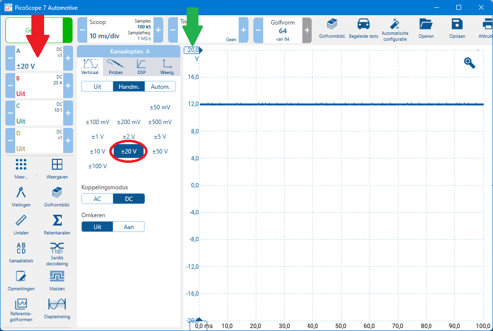
When the measured voltage is higher than the set voltage of (in this case) 20 volts, the message “channel overrange” will appear at the top of the screen. The voltage scale then needs to be increased. Using the arrows to the left and right of the menu button, the voltage can be increased or decreased step by step without opening the menu.
Picoscope: setting the time per division:
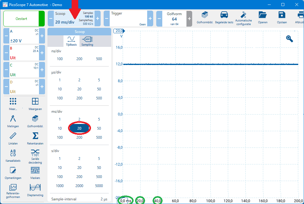
After setting the voltage to a maximum of 20 volts, the time per division can be set. To set this time, we click the button for the time setting (next to the red arrow). In the menu that appears, we select the desired time per division. In the image, 5 ms/div is circled.
After clicking 20 ms/div, you see the time at the bottom on the X-axis increase for each division, starting from 0.0 up to 200.0 ms. The times 0, 20 and 40 ms are circled in green in this example.
The time setting depends on which component, system or process we want to measure;
- battery voltage while cranking or a relative compression test: 1 second per division;
- signal from sensors and actuators: 10 to 100 ms/div.
During the measurement the time base can be adjusted to display a correct signal on the screen.
Picoscope: setting the trigger:
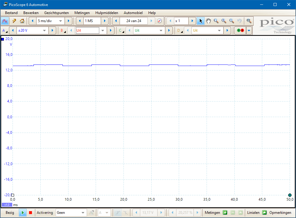
Constant voltages, such as the system voltage in the earlier examples, can also be measured with a standard multimeter. Non-constant voltages, such as a strongly varying signal voltage from a sensor or a PWM control signal, cannot or hardly be displayed by a voltmeter. In the case of a PWM or duty cycle, a voltmeter will show an average value. We measure such voltages with the oscilloscope. The scope image below shows the PWM control of an interior blower motor. Without a trigger setting, the image keeps jumping across the screen.
The square-wave voltage constantly jumps across the screen. A change in pulse width cannot be observed properly. To lock the voltage on the screen while still measuring in real time (with pause enabled, no change is visible), we use the trigger. In the Picoscope software, the Trigger function can be found as a button among the settings at the top. In the image below the button is indicated with a red arrow. By default it shows “None”, meaning no trigger is being used.
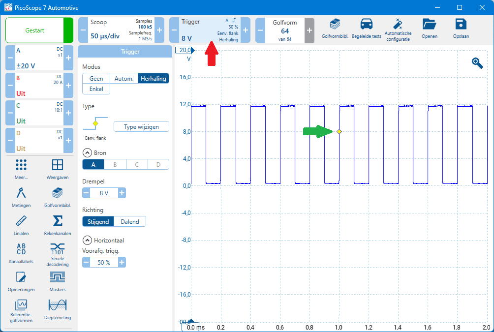
The next image shows the signal with the trigger enabled. Here the mode “Repeat” is selected. A yellow dot appears on the screen; this is the point at which the trigger occurs. In this case, the green arrow points to the trigger. Using the mouse we can move this point to any other place within the voltage range.
After setting the trigger, changes in the PWM signal can be observed at the moment the conditions change: the sensor passes on a change in the signal, or the actuator is activated more or less by the ECU. In the image below we see a PWM signal in which the ground-side control becomes wider and narrower.
When measuring the signal, it may also be desirable to trigger on the negative edge; for example, when measuring the voltage pattern of an injector because that is the point where the control begins. Set it as follows: click the “advanced triggers” button (red arrow in the image). A new window opens where, under “simple edge”, you can change the direction from “rising” to “falling” (blue arrow). From that moment on, the trigger point in the signal is on the negative edge (green arrow).
The following example shows the voltage pattern of an injector. Just like with the PWM control voltage of the interior fan in the previous example, this signal jumps across the screen when no trigger is used. In the example, the trigger is set to the falling edge of channel B. In the “Trigger” button, B is highlighted in red with a Z symbol, which indicates the negative edge.
After setting the trigger point, the signal is fixed on the screen (see image below). The signal has a fixed starting point: the control begins where the injector is switched to ground. During acceleration, enrichment takes place: the injector is opened for a longer period of time to inject more fuel. In that case, the ECU switches the injector to ground for a longer time span.
During deceleration, fuel injection stops: in that case, the injector is not switched to ground. The voltage then remains constant (approximately 14 volts). Because in this measurement we have set the trigger on the falling edge, deceleration is not clearly visible. Only after disabling the trigger do we see that the voltage remains at 14 volts, but as soon as injection is resumed, the trace will again jump across the screen.
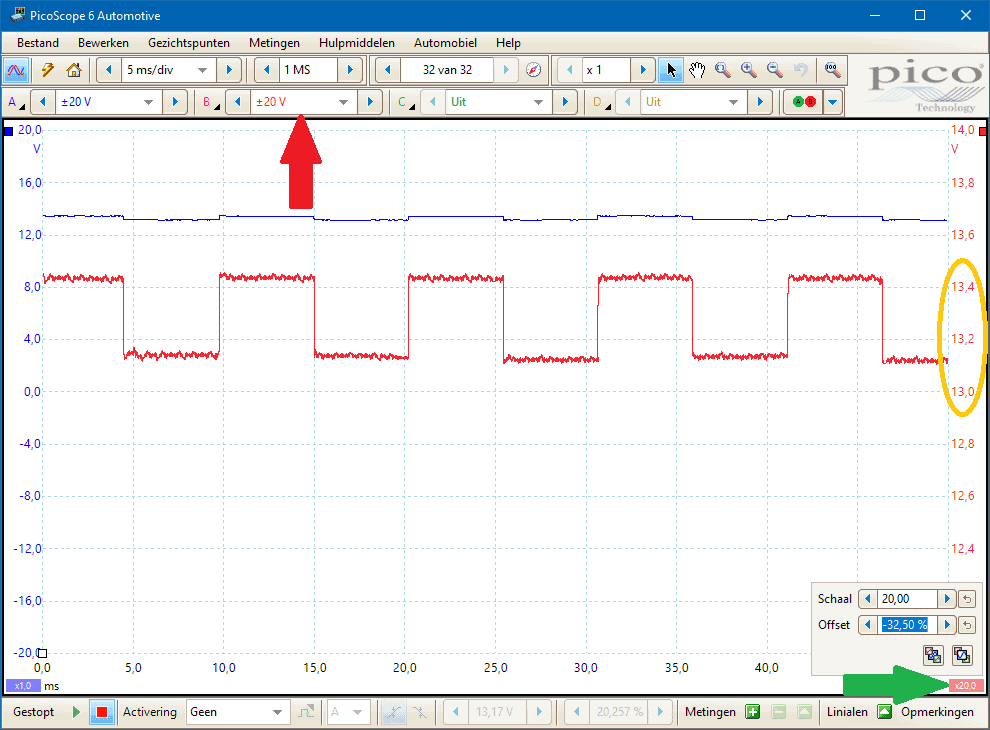
Picoscope: scale and offset:
The square-wave signal of an ABS sensor (Hall) has a small voltage difference. The oscilloscope image below shows the trace that is measured directly on the ABS sensor. Inside the ABS control unit there is a circuit that amplifies the voltage difference. For diagnosing the ABS sensor, this oscilloscope image is not clear enough. By changing the scale and offset, the signal can be magnified.
In the measurement below, channel B is connected to the same wire as channel A. The measurement is identical, but due to the different settings the signal is displayed more clearly. The green arrow indicates one of the places where you can change the scale and offset.
- The scale zooms in on the signal: we are now measuring within the voltages 12 and 14 volts.
- The offset can be adjusted to position the signal at the correct height on the screen. With an offset of 0%, the voltage on the Y-axis between 0 and 2 volts is visible.
Fluke introduction:
The image alongside shows a Fluke 123 handheld oscilloscope, which is used in car workshops, test and development areas, and in education. Although there are different brands, they often look very similar and work almost the same. On top of the oscilloscope there is a red and a grey input, which are called channels A and B respectively. In the middle is the ground connection.
The oscilloscope can display two measurements simultaneously on one screen (A and B separately), as can also be seen in the image. Measurement A is shown at the top and measurement B at the bottom, making it easy to compare signals from two different sensors. For a single measurement, channel A is used by default.
The oscilloscope can measure both DC and AC voltage. In automotive applications we use the DC mode to measure DC voltages.
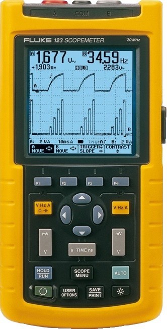
In the image, the battery voltage is being measured. Between the zero line (the black dash at the bottom left) and the measured voltage (the thick line above “A”) seven squares are visible. Each square is called a division.
Unlike with the Picoscope, you do not set the total voltage range, but the voltage per division. The voltage setting per division is set to 2 V/d (bottom left on the screen). This means that each square represents 2 volts. Because there are seven squares between the zero line and the signal, the voltage can easily be calculated: 7 × 2 = 14 volts. The average voltage is also shown on the screen (14.02 volts).
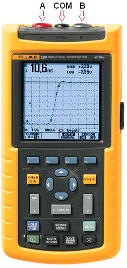
Press the green button at the bottom left to switch on the oscilloscope. For a measurement, place the red test probe in channel A and the black test probe in the COM connection.
To measure a signal, connect the red test probe (channel A, positive) to the signal terminal of the sensor or to the correct point in the break-out box. Connect the black test probe (COM) to a good ground point on the bodywork or to the battery negative terminal. For a single voltage measurement, only channel A and the COM connection are required.
When two voltage signals need to be compared, use channel B. In that case, place the test probe in input B and switch on channel B on the oscilloscope.
The oscilloscope has an “AUTO” button. This function ensures that the oscilloscope automatically selects the best settings for the input signal. A disadvantage is that the signal is not always displayed correctly; the oscilloscope may constantly adjust the settings with a signal that has a variable amplitude (height) and frequency (width). Comparing voltage signals with different time settings can then become difficult. Therefore, it is better to set up the oscilloscope manually and perform multiple measurements with the same settings. The following paragraphs explain how to do this.
Fluke: setting the zero line:
After switching on the Fluke oscilloscope, the zero line is often automatically placed in the middle of the screen. With a setting of 1 volt per division, the range is then only 4 volts above and 4 volts below the zero line. As a result, a voltage higher than 4 volts will not fully fit on the screen and the line will run off-screen. To make the full voltage range visible, the zero line must be moved downwards. In the image, the zero line is set to the bottom line of the screen.
With the zero line at the bottom and the setting at 1 V/d, the oscilloscope can display a maximum voltage of 8 volts (8 × 1 = 8 V). This is suitable for measuring the supply voltage or signals from active sensors (maximum 5 volts), but insufficient for higher voltages such as the battery voltage or the voltage across a lamp. For that, 2 V/d (passenger cars) or 5 V/d (commercial vehicles) is an appropriate setting.
Fluke: setting voltage and time per division:
As discussed earlier, the number of volts per division must be set correctly to keep the voltage signal within the screen. The correct setting of the time per division is also essential. This paragraph describes how to adjust both settings.
If the number of volts per division is too low, the measurement will fall outside the screen. If the number of volts per division is too high, only a small signal is visible. For an optimal measurement, the signal should make full use of the screen.
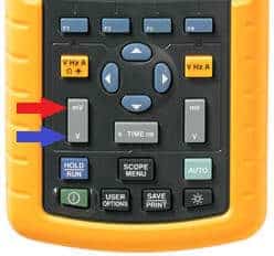
In the image, the number of volts per division is adjusted with the button labelled “mV” and “V”. By pressing “mV” (red arrow), you reduce the volts per division, and by pressing “V” (blue arrow), you increase it.
By setting the time per division, the duration of the measurement can be adjusted. With a setting of 1 second per division (1 s/d), the line moves one square every second. This is also visible in the voltage graph, where the line moves one division from left to right every second. Depending on the type of measurement, it is desirable to adjust the time setting. When measuring the voltage curve of an injector, the time setting must be lower than when measuring a duty cycle.
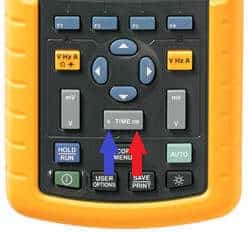
The time setting can be increased by pressing the “s” on the left side of the “TIME” button and decreased with the “ms” button. The time setting applies to both channel A and B; it is not possible to use different time settings for channels A and B.
Fluke: setting the trigger:
When measuring voltages such as the battery voltage, a trigger is not required. The battery voltage (as described in the paragraph “General”) appears as a straight line, where you count the divisions between the zero line and the signal. This line remains constant, unless the battery is being charged or a consumer is switched on, causing the voltage to drop over time.
However, when measuring a sensor signal, the voltage line will not be constant and its height will shift across the screen. Although the HOLD button can be used to temporarily freeze the image for closer inspection, this is not ideal. The button has to be pressed at exactly the right moment, and once frozen, the screen no longer shows any changes in the signal. The trigger function offers a solution: by setting the trigger, the voltage signal is held at a certain point on the screen. The measurement continues, so changes in the signal remain visible when conditions change, such as fluctuations in engine speed or temperature.
The trigger symbols are as follows:
Trigger for the rising edge. This trigger function freezes the waveform at a point where it is going up.
Trigger for the falling edge. This is the opposite symbol of the rising edge. This trigger function freezes the waveform when it first goes down.
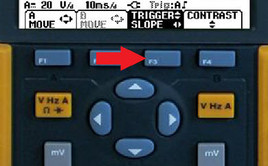
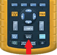
Press the F3 button (see image) to move the trigger. Move the trigger up and down with the arrow keys. Change the trigger from rising to falling edge with the left and right arrows.
In the two images below, the same waveform is shown with two different trigger settings.
Trigger on the rising edge:
In the image, the trigger is shown on the rising edge of the signal. As a result, the oscilloscope will keep the image stationary as long as the sensor signal is being measured. If the trigger were not set, this signal would continuously scroll across the screen from left to right.
Trigger on the falling edge:
Here, with the same measurement, the trigger is set on the falling edge. This image clearly shows that the trace is the same, but that the signal has shifted slightly to the left. With this trigger function, the image is held at the point where it goes down.
Of course, the trigger is not a way to pause the screen. As soon as the measured object is switched off or when the signal changes, the trace on the screen will change along with it.
This can be seen in the image; the trigger is at the same point, but the horizontal voltage line has become more than twice as long. The voltage of 1.5 volts (1500 mV) is now active for 110 µs (microseconds) instead of 45 µs in the previous measurement.
Fluke: switching the smooth function on or off:
Because the oscilloscope is very precise, some noise will always be visible in the trace. This can be distracting, especially when an accurate assessment of the voltage signal is required. To clean up the trace and reduce noise, the “smooth” function can be switched on.
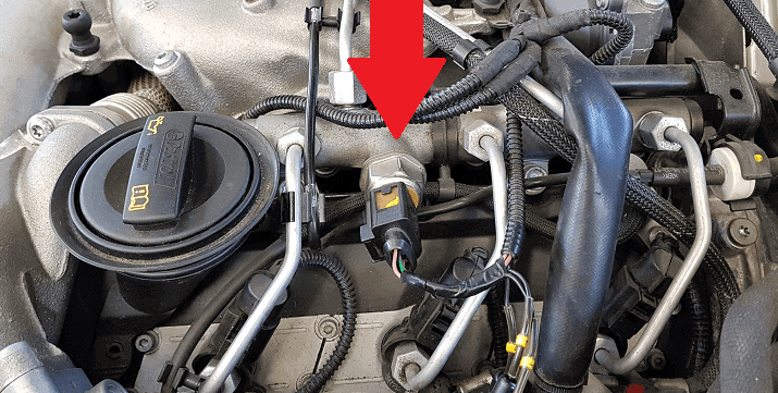
The following measurement was taken at the signal output of the fuel pressure sensor located on the fuel rail of the injectors of a common-rail diesel engine (indicated by the red arrow in the image alongside).
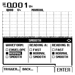
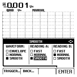
In the screenshots below you can clearly see a difference between the traces with Smooth switched off and on.
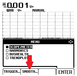
The Smooth function can be set by performing the following three steps via the settings menu that appears after pressing the “Scope menu” button:
Fluke: enabling channel B:
When measuring signals, it is often desirable to measure two signals relative to each other, for example the camshaft signal and the crankshaft signal in relation to time. The voltage curves of both sensors are then neatly displayed one below the other, allowing conclusions to be drawn about the timing of the valve train.
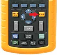
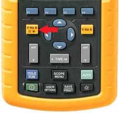
To enable channel B, press the yellow button on the right side of the oscilloscope. As soon as the menu appears on the screen, use the arrow keys to select the desired option. Confirm the selection with the F4 button, which is labeled “ENTER” above it. Channel B can be switched off again in the same way.
In the images below you can see the menu that appears after pressing the yellow button. In the left-hand menu, “OFF” is selected under B. With the arrow keys this can be changed to “ON”. Next, the “Vdc” option (direct voltage) must be selected, as shown in the image on the right. After each option has been confirmed with “ENTER,” the menu disappears and measurements can be taken with channel B.
After enabling channel B, the zero line must be set to the desired position, just as with channel A. The time settings per division are the same for both channels: it is not possible to have the voltage curve of channel A and B differ from each other.
Fluke: measuring with the current clamp:
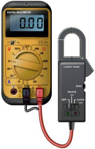
With the oscilloscope, only voltages can be measured. Even when measuring current with a current clamp, the oscilloscope will receive a voltage signal from the clamp. This paragraph explains how to take measurements with the current clamp. To make it easier to understand, we will first look at an example using the multimeter.
The current clamp can also be used in combination with a multimeter. Inside the current clamp there is a Hall sensor that measures the magnetic field passing through the jaws of the clamp. This magnetic field is converted into a voltage up to 5 volts.
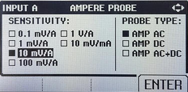
Where the internal fuse of the multimeter can fail at currents higher than 10 Amps, the current clamp can measure currents of hundreds of Amps. The voltage supplied by the current clamp is 100 times smaller than the actual current, due to the conversion factor of 10 mV/A, which is also indicated on the clamp. Make sure that the clamp is set to the first position and not to 1 mV/A (conversion factor 1000).
When the current clamp is connected to the volt input of the multimeter and the clamp is switched on and calibrated until the multimeter reads 0 volts, the clamp can be placed around the cable of the sensor or actuator. When reading the multimeter, the conversion factor must be taken into account: each millivolt indicated by the multimeter represents 1 Amp.
It is easy to remember that the measured value must be multiplied by a factor of 100. For example, if the display shows 0.25 volts, the actual current is (0.25 * 100) = 25 Amps. If during another measurement the display shows 1.70 volts, then the actual current is also one hundred times higher, so 170 Amps. In short, the decimal point is moved two places to the right.
The previous example was measuring with the multimeter, because in that case measuring with the scope may be a bit easier to recognize. The same current clamp can also be connected to the oscilloscope. The red and black leads of the current clamp must be plugged into channel A (or B) and the COM connection of the clamp.
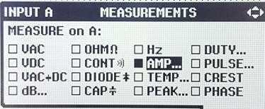
At this point, the oscilloscope is set to Amps. First calibrate the current clamp by turning the calibration knob until the oscilloscope indicates 0 A.
When the current clamp outputs a voltage of 0.050 volts, the oscilloscope automatically converts this value using a factor of 100, because every 10 mV corresponds to 1 Ampere in reality. The display of the oscilloscope will then show 5 Amps.
The current clamp is very fast and makes it possible to measure even the current waveform of an injector. With the oscilloscope’s two-channel function, the voltage waveform can be measured on channel A and the current waveform on channel B. The voltage and current waveforms are neatly displayed one below the other.